Laboratory X-ray Powder Data - Fluroapatite

A video version of this tutorial is available at https://anl.box.com/v/LaboratoryX-

Exercise files are found here

In this tutorial you will refine the structure of fluoroapatite, Ca₅F(PO₄)₃, using constant wavelength laboratory X-ray powder diffraction data. At the completion of the refinement you will then prepare a drawing of the fluoroapatite structure. The structure is hexagonal with four different kinds of atoms spread over seven different sites. The data was taken on a conventional Bragg-Brentano powder diffractometer using CuK_a radiation.

If you have not done so already, start GSAS-II.

We suggest that you do the Neutron CW Powder Data exercise first before doing this one. Some things are covered there in more detail that we will not cover here.

Step 1: read in the data file

1. Use the Import/Import Powder Data/from GSAS powder data file menu item to read the data file into GSAS-II. This option reads all of the powder data formats (except neutron TOF time map files) used in the GSAS program (with angles in centidegrees). If the data files are not downloaded with the tutorial, download them from https://subversion.xray.aps.anl.gov/pyGSAS/Tutorials/LabData/data/) otherwise, if needed, change the file directory to LabData/data to find the file; you will need to change the file type to any file (*.*) to find the desired file.

2. Select the FAP.XRA data file in the first dialog and press Open. There will be a Dialog box asking Is this the file you want? Press Yes button to proceed.

3. Select the INST_XRY.PRM instrument parameter file in the second dialog and press Open.

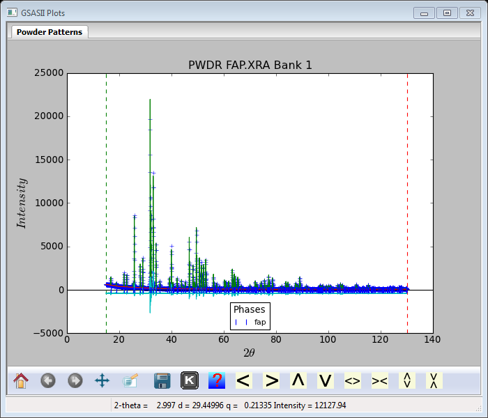
At this point the GSAS-II data tree window will have several entries and the plot window will show the powder pattern

Step 2: Create the phase

For this step we will take advantage of having an old GSAS experiment file with all the parameters for fluroapatite otherwise you’ll have to follow the steps used for the CW neutron example on garnet with the following information:

Phase name = ‘fap’, Space group = P 63/m, unit cell a = 9.372, c = 6.886

Atom coordinates:

TYPE	X	Y	Z
Ca	0.333333	0.666667	0.001
Ca	0.242	0.992	0.25
P	0.397	0.367	0.25
F	0.0	0.0	0.25
O	0.325	0.485	0.25
O	0.591	0.469	0.25
O	0.340	0.258	0.07

To import the fluroapatite phase information from the file FAP.EXP use the Import/Import Phase menu to see a pulldown menu. Select from GSAS .EXP file. The file selection dialog will still be set to the directory the data was found; click on FAP.EXP and Open to open it. You will see an Is this the file you want? dialog; press Yes to proceed. A small dialog box with a phase name of ‘fap’ will appear. We didn’t change it so press OK to accept it. Next an Add histogram(s) dialog will appear; select the PWDR FAP.XRA item and press OK.

Step 3 First view of the general phase information

The GSAS-II data tree should now have a Phase entry of fap; the fap phase information will be shown

You can see that the number of each kind of atom gives 2 formula units per cell. The Data tab will show the sample broadening information, etc. associated with the powder data set we just loaded.

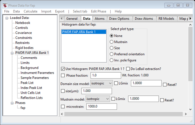
We will return to this window later when we consider the effect of crystallite size and mustrain broadening.

Step 4: Adjust background parameterization

You may have noticed that the background in this powder pattern rises significantly at low angles; there is also a less apparent rise at the high angle end as well. The default background function doesn’t handle this very well so find the Background item under PWDR FAP.XRA: BANK1 in the GSAS-II data tree and press it. The Background window will appear

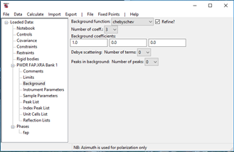
Change the background function to log interpolate and the number of coefficients to 9. This will put background points at the two limits and at equal spaces in log(2Q) in between so there are more where the background is changing most rapidly. A linear interpolation is then used to compute the background for all points in the pattern during the Rietveld refinement.

Step 5 1^st Rietveld refinement

You are now ready for the 1^st Rietveld refinement; the histogram scale (found in Sample Parameters) and background will be refined. Press Calculate/Refine in the GSAS-II data tree menu. You will be asked for a project file name, we used ‘fap’ and made the file fap.gpx. The refinement proceeds and when complete (Rwp ~45.2%) a small dialog box will appear asking Load new result? Press OK; the windows will be updated and a new plot is displayed.

Expanding the plot shows that much of the difference is that the calculated peaks are out of place. This is due to lattice parameters and also that in this Bragg-Brentano experiment the sample position is offset from the focusing circle. Important: this is the most likely reason for peaks displacement errors in laboratory data, not the zero point. The lattice parameter flag (this is the checkbox next to the lattice parameters determines if the lattice parameters will be refined and is called the refinement flag) is on the General tab for the Phase fap and the sample displacement is found on the Sample Parameters item under PWDR FAP.XRA: BANK1 in the GSAS-II data tree. Go to both places and set those flags (checkboxes); make sure that the Diffractometer type is Bragg-Brentano.

Step 6 2^nd Rietveld refinement

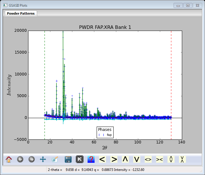
Now do the Rietveld refinement by Calculate/Refine menu on GSAS-II data tree window. The plot will be

noticeably improved (Rwp ~14.5%). Close inspection (see inset) shows that most of the differences are in the widths of the peaks so we should refine crystallite size and mustrain parameters next.

Step 7 3^rd Rietveld refinement

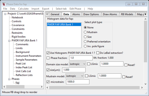
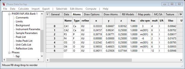
Select the Phases/fap item in the GSAS-II data tree and then select the Data tab and set the refine flags for both size and mustrain. The window should look like

Now do the refinement; press the Calculate/Refine menu item on the GSAS-II data window. Do not be alarmed about how the Rwp jumps around on the progress bar; that is a consequence of how the Levenberg-Marquardt algorithm does a least squares minimization. The result in the end is noticeably better than before (Rwp=11.2%)

Step 8. 4^th Rietveld refinement

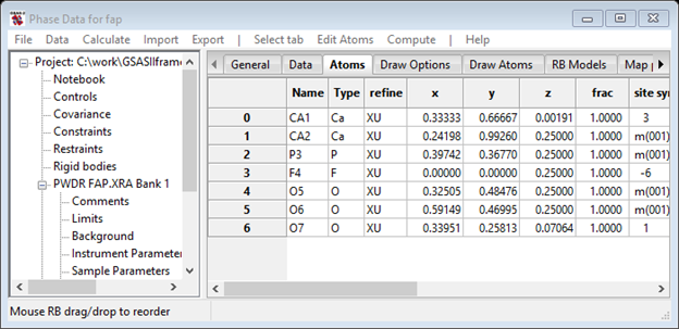
Now we can refine atom parameters. Select Phases/fap and the Atoms tab; the Phase data for fap window will display

Double click the refine column header; a new window will show Refinement controls

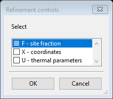
Select X - coordinates and U - thermal parameters and press OK. The Atoms tab will show new refine flags

Now run the refinement; press the Calculate/Refine menu item on the GSAS-II data tree window. The result is a bit better (Rwp=10.4%) and the plot is pretty much the same as before

and the atom parameters are

The refinement is now essentially complete. The file fap.lst has the result of the last cycle of refinement with values and esds for all the parameters

Refinement results:

---------------------------------------------------------------------------------------------------------------------------------------

Number of function calls: 12 Number of observations: 5751 Number of parameters: 34

Refinement time = 12.605s, 3.151s/cycle, for 4 cycles

wR = 10.38%, chi**2 = 19687.8, reduced chi**2 = 3.44

----------------------------------------------------------------------------------------------------------------------------------

Variables generated by constraints

name : 0::A0

value : 0.0152

sig : 0.0000

Phases:

Result for phase: fap

Reciprocal metric tensor:

names : A11 A22 A33 A12 A13 A23

values: 0.015180436 0.015180436 0.021090011 0.015180436 0.000000000 0.000000000

esds : 0.000000320 0.000000255

New unit cell:

names : a b c alpha beta gamma Volume

values: 9.371891 9.371891 6.885914 90.0000 90.0000 120.0000 523.777

esds : 0.000189 0.000042 0.008

Atoms:

name x y z frac Uiso U11 U22 U33 U12 U13 U23

---------------------------------------------------------------------------------------------------------------------------------------

CA1 Ca:

values: 0.33333 0.66667 0.00202 1.000 0.00840

sig : 0.00030 0.00036

CA2 Ca:

values: 0.24161 0.99231 0.25000 1.000 0.00712

sig : 0.00016 0.00019 0.00029

P3 P:

values: 0.39715 0.36781 0.25000 1.000 0.00719

sig : 0.00020 0.00019 0.00040

F4 F:

values: 0.00000 0.00000 0.25000 1.000 0.01746

sig : 0.00142

O5 O:

values: 0.32546 0.48503 0.25000 1.000 0.00814

sig : 0.00043 0.00044 0.00105

O6 O:

values: 0.59033 0.46939 0.25000 1.000 0.01114

sig : 0.00045 0.00048 0.00112

O7 O:

values: 0.33975 0.25900 0.07097 1.000 0.01096

sig : 0.00035 0.00035 0.00035 0.00079

Phase: fap in histogram: PWDR FAP.XRA Bank 1

----------------------------------------------------------------------------------------------------------------------------------

Final refinement RF, RF^2 = 3.32%, 7.53% on 325 reflections

Bragg intensity sum = 1.16e+06

Size model: isotropic equatorial: 0.39088, sig: 0.0718 LG mix coeff.: 1.0000

Mustrain model: isotropic equatorial: 961.3, sig: 25.8 LG mix coeff.: 1.0000

Histogram: PWDR FAP.XRA Bank 1 histogram Id: 0

---------------------------------------------------------------------------------------------------------------------------------------

PWDR histogram weight factor = 1.000

Final refinement wR = 10.38% on 5751 observations in this histogram

Other residuals: R = 8.12%, Rb = 8.36%, wRb = 10.23% wRmin = 5.61%

Instrument type: Bragg-Brentano

Sample Parameters:

names : Scale Shift Transparency SurfRoughA SurfRoughB

values: 42.2873 83.9821 0.0000 0.0000 0.0000

sig : 0.1442 0.3609

Background function: log interpolate

value : 623.5 405.2 262.1 154 104.5 71.38 50.48 49.97 59.71

sig : 5.36 3.124 2.364 1.785 1.334 1.016 0.9211 1.141 1.451

Background sums: empirical 6.3e+05, Debye 0, peaks 0, Total 6.3e+05

Step 9. Draw the structure

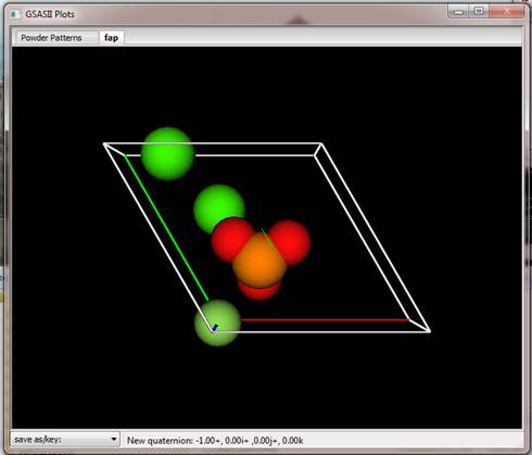
What we like to show is the unit cell contents with the PO₄^-3 ions as tetrahedra and the Ca and F atoms as balls. Begin by finding Phases/fap in GSAS-II data tree and selecting the Draw Options tab. The Phase data for fap window shows Drawing Options

The plot will show a new tab marked fap showing some balls in various colors. A unit cell box is drawn with 3 colored edges (Red, Green & Blue for a, b, c axes, respectively). A multicolored (RGB, again) 3D cross is at the center of the plot.

Notice the slider controls in Drawing controls; you can change them to change the how the structure is displayed. Press the Draw Atoms tab; this will show the list of atoms that are drawn in the picture.

This is a copy of what is in the Atoms table; there are columns that allow you to change how the atoms are displayed, their labels and their color all controlled on an atom-by-atom basis. Now if the contents of the Atoms table change (e.g. by refinement) then you must manually update the Draw Atoms table by erasing all the Draw Atoms. They are then automatically refreshed from the Atoms table with the new values. Do this by selecting all the Draw Atoms; double click the blank in the upper left corner of the table. All atoms will be highlighted in dark gray; they will all be green on the plot. Then press Edit/Delete atoms in the Draw Atoms menu. All the atoms will vanish and then reappear with updated values. Now we can draw the structure assured that we are using the final result from the refinement.

To build the structure model we want to show with PO₄ tetrahedra and balls for the F and Ca atoms in a unit cell box (the box should already be visible) do the following steps:

1. Select all the atoms in the Draw Atoms tab by double clicking in upper left corner box of the table. All atoms in the table are then displayed in dark gray and they all are green on the drawing indicating their selection.

2. Select Edit Figure/Fill unit cell from the menu. The drawing will show the unit cell filled with atoms in positions equivalent to the original set and the Draw Atoms table will have all of them listed. The Sym Op column in the table shows the symmetry operator number and unit cell translation used to generate that position.

3. Double click on the column label Type. A small dialog window will appear with a list of element types in this structure. Select P by checking the box and then press OK. All the P atoms will be bright green and they will be highlighted in dark gray in the table

4. Select Edit Figure/Fill CN-sphere in the menu. Each P atom will now have its full complement of 4 O atoms.

5. Repeat step 3 to select all the P atoms again.

6. Select Edit Figure/Atom style from the Draw Atoms menu. A small dialog bow will appear with a list of possible atom drawing styles. Notice the first one is blank; that will cause the atom to not be drawn. Select polyhedra and press OK. Each P atom will be drawn as a brass colored polyhedron (with too many faces to be a tetrahedron because a nearby Ca atom was included – this will be fixed in a moment).

7. Now do step 3 yet again but this time select the O atoms.

8. Select Edit Figure/Atom style and pick the blank entry and press OK; the O atoms will vanish leaving some odd polyhedra and the Ca and F atoms.

9. Select the Drawing Options tab and change the Bond search factor to 0.80 and press Enter; the odd polyhedra will immediately change to tetrahedra.

10. You can adjust the van der Waals scale to make all the balls any size you desire.

11. If you don’t like the fact that both Ca and F are in a very similar green, you can change this. Select the Draw Atoms tab, then do step 3 selecting the Ca atoms.

12. Select Edit/Atom color in the Draw Atoms menu. A color selection dialog box will appear (NB: this dialog is operating system dependent – we will assume you are using a Windows7 machine). The dialog box looks like (I pressed Define Custom Colors)

The steps for changing a color is to either a) choose your color by finding it in Basic colors and then press OK or b) press Define Custom Colors, move the cross around on the spectrum display, set the vertical slider for the luminosity (ColorSolid will show the result), and then press OK. The drawing will now show that color for the atoms and the color will appear in the Draw Atoms table. If you don’t like your colors select Edit/Reset atom colors to put them back to their default colors. In my drawing I’ve made the Ca atoms a medium gray

Step 10. Calculate bond distances and angles

GSAS-II will compute all the distances and angles among all the atoms you select in the Atoms table with controls on the range of atom-atom distances to consider either globally or by atom type.

1. To start select the Atoms tab in Phases/fap.

2. Select the first Ca atoms by clicking on its row label (an “0”). Add to the selection the other Ca atom and the P atom in the same way with the Ctrl key down; all will be highlighted in blue.

3. Select Compute/Show Distances & Angles from the Atoms menu. A small dialog box will appear

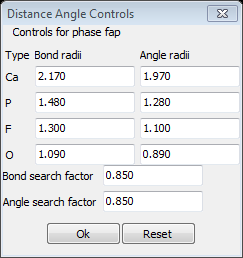
Here you have individual controls on various atom radii to consider for both distance and angle calculations as well as global search factors. Considering our experience with drawing the PO₄ tetrahedra the Bond and Angle search factors may be too large for this case. Change both to 0.8 and press OK. GSAS-II will then display on the console formatted tables of individual atom distances and angles with esds as appropriate for the two Ca atoms and the P atom.

********************************************************************************

Interatomic Distances and Angles for phase fap

********************************************************************************

Space Group: P 63/m

The lattice is centrosymmetric primitive hexagonal

The Laue symmetry is 6/m

The lattice point group is 6/m

Multiplicity of a general site is 12

The inversion center is located at 0,0,0

The equivalent positions are:

( 1) X, Y, Z ( 2) X-Y, X, 1/2+Z

( 3) -Y, X-Y, Z ( 4) -X, -Y, 1/2+Z

( 5) Y-X, -X, Z ( 6) Y, Y-X, 1/2+Z

Unit cell: a = 9.37189(19) b = 9.37189 c = 6.88591(4) alpha = 90 beta = 90 gamma = 120 Volume = 523.777(8)

Distances & angles for CA1 at 0.33333 0.66667 0.00202

********************************************************************************

To cell +(sym. op.) dist. CA1 CA1 CA1 CA1 CA1 CA1

O6 O6

CA1 [ 0 1 0] +( -2) 3.471(4)

CA1 [ 0 1 1] +( -2) 3.415(4)

CA1 [ 0 0 0] +( -4) 3.471(4)

CA1 [ 0 0 1] +( -4) 3.415(4)

CA1 [ 1 1 0] +( -6) 3.471(4)

CA1 [ 1 1 1] +( -6) 3.415(4)

O5 [ 0 0 0] +( 1) 2.3860(28)

O5 [ 1 1 0] +( 3) 2.3860(28)

O5 [ 0 1 0] +( 5) 2.3860(28)

O6 [ 0 0-1] +( 2) 2.4620(31)

O6 [ 1 1-1] +( 4) 2.4620(31)

O6 [ 0 1-1] +( 6) 2.4620(31)

Distances & angles for CA2 at 0.24161 0.99231 0.25

********************************************************************************

To cell +(sym. op.) dist. F4 O6 O7 O7 O7

F4 [ 0 1 0] +( 1) 2.3012(11)

O6 [ 1 1 0] +( 3) 2.350(4)

O7 [ 0 1 0] +( 1) 2.5128(30)

O7 [ 0 1 0] +( 6) 2.3434(24)

O7 [ 0 1 0] +( -3) 2.3434(24)

O7 [ 0 1 1] +( -4) 2.5128(30)

Distances & angles for P3 at 0.39715 0.36781 0.25

********************************************************************************

To cell +(sym. op.) dist. O5 O6 O7

O5 [ 0 0 0] +( 1) 1.548(4)

O6 [ 0 0 0] +( 1) 1.569(4) 110.37(23)

O7 [ 0 0 0] +( 1) 1.5167(27) 110.07(15) 108.77(15)

O7 [ 0 0 1] +( -4) 1.5167(27) 110.07(15) 108.77(15) 108.74(23)

There is probably too many bonds shown for the Ca1 atom and no angles given; you can repeat the calculation with somewhat smaller Ca radii to fix this. Setting the Bond and Angle Ca radii to 2.1 and 1.9, respectively, and the Angle search factor to 0.95 gave

********************************************************************************

Interatomic Distances and Angles for phase fap

********************************************************************************

Space Group: P 63/m

The lattice is centrosymmetric primitive hexagonal

The Laue symmetry is 6/m

The lattice point group is 6/m

Multiplicity of a general site is 12

The inversion center is located at 0,0,0

The equivalent positions are:

( 1) X, Y, Z ( 2) X-Y, X, 1/2+Z

( 3) -Y, X-Y, Z ( 4) -X, -Y, 1/2+Z

( 5) Y-X, -X, Z ( 6) Y, Y-X, 1/2+Z

Unit cell: a = 9.37189(19) b = 9.37189 c = 6.88591(4) alpha = 90 beta = 90 gamma = 120 Volume = 523.777(8)

Distances & angles for CA1 at 0.33333 0.66667 0.00202

********************************************************************************

To cell +(sym. op.) dist. O5 O5 O5 O6 O6

O5 [ 0 0 0] +( 1) 2.3860(28)

O5 [ 1 1 0] +( 3) 2.3860(28) 74.44(11)

O5 [ 0 1 0] +( 5) 2.3860(28) 74.44(11) 74.44(11)

O6 [ 0 0-1] +( 2) 2.4620(31) 124.40(11) 154.16(12) 92.77(9)

O6 [ 1 1-1] +( 4) 2.4620(31) 92.77(9) 124.40(11) 154.16(12) 75.80(12)

O6 [ 0 1-1] +( 6) 2.4620(31) 154.16(12) 92.77(9) 124.40(11) 75.80(12) 75.80(12)

Distances & angles for CA2 at 0.24161 0.99231 0.25

********************************************************************************

To cell +(sym. op.) dist. F4 O6 O7 O7 O7

F4 [ 0 1 0] +( 1) 2.3012(11)

O6 [ 1 1 0] +( 3) 2.350(4) 152.07(12)

O7 [ 0 1 0] +( 1) 2.5128(30) 81.10(7) 74.63(11)

O7 [ 0 1 0] +( 6) 2.3434(24) 102.85(8) 85.36(8) 135.15(12)

O7 [ 0 1 0] +( -3) 2.3434(24) 102.85(8) 85.36(8) 77.50(6) 141.17(14)

O7 [ 0 1 1] +( -4) 2.5128(30) 81.10(7) 74.63(11) 58.76(12) 77.50(6) 135.15(12)

Distances & angles for P3 at 0.39715 0.36781 0.25

********************************************************************************

To cell +(sym. op.) dist. O5 O6 O7

O5 [ 0 0 0] +( 1) 1.548(4)

O6 [ 0 0 0] +( 1) 1.569(4) 110.37(23)

O7 [ 0 0 0] +( 1) 1.5167(27) 110.07(15) 108.77(15)

O7 [ 0 0 1] +( -4) 1.5167(27) 110.07(15) 108.77(15) 108.74(23)

which is probably more reasonable.

This concludes this tutorial for Rietveld refinement of fluroapatite.